|
1 2 3 4 5 6 7 8 9 10 11 12 13 14 15 16 17 18 19 20 21 22 23 24 25 26 27 28 29 30 31 32 33 34 35 36 37 38 39 40 41 42 43 44 45 46 47 48 49 50 51 52 53 54 55 56 57 58 59 |
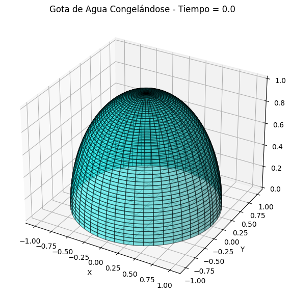
import numpy as np import matplotlib.pyplot as plt from mpl_toolkits.mplot3d import Axes3D def esfera_mitad(r, phi, theta): """Genera las coordenadas cartesianas para la mitad superior de una esfera.""" x = r * np.sin(theta) * np.cos(phi) y = r * np.sin(theta) * np.sin(phi) z = r * np.cos(theta) return x, y, z # Parámetros del modelo r0 = 1 # Radio inicial de la gota en unidades arbitrarias T0 = 100 # Temperatura inicial de la gota en °C T_amb = 0 # Temperatura ambiente en °C k = 0.05 # Constante de congelación t_max = 50 # Tiempo máximo de simulación h = 5 # Paso de tiempo # Inicializar el tiempo y el radio num_steps = int(t_max / h) + 1 t = np.linspace(0, t_max, num_steps) r = np.zeros(num_steps) r[0] = r0 # Método de Euler para resolver la ecuación diferencial for i in range(1, num_steps): dR_dt = -k * (T0 - T_amb) # Cambio en el radio por unidad de tiempo r[i] = r[i - 1] + h * dR_dt # Asegurarse de que el radio no sea negativo if r[i] < 0: r[i] = 0 # Crear una malla de coordenadas esféricas phi, theta = np.mgrid[0:2*np.pi:100j, 0:np.pi/2:50j] # Solo la mitad superior (0 a pi/2) # Crear la figura y el eje 3D fig = plt.figure(figsize=(14, 7)) ax = fig.add_subplot(111, projection='3d') # Graficar la esfera para cada instante de tiempo for i in range(num_steps): # Radio en el instante de tiempo i radius = r[i] # Coordenadas cartesianas de la esfera x_sphere, y_sphere, z_sphere = esfera_mitad(radius, phi, theta) # Graficar la esfera ax.clear() ax.plot_surface(x_sphere, y_sphere, z_sphere, color='cyan', alpha=0.5, edgecolor='k') ax.set_title(f'Gota de Agua Congelándose - Tiempo = {t[i]:.1f}') ax.set_xlabel('X') ax.set_ylabel('Y') ax.set_zlabel('Z') ax.set_zlim(0, 1) # Ajustar el límite del eje Z para centrarse en la mitad superior plt.pause(0.1) # Pausa para la animación plt.show() |